
Project Gutenberg is a website that offers more than 58,000 free eBooks for which U.S. copyright have expired. It is very interesting text data for Natural Language Processing (NLP), as it is a huge body of text with pretty reliable labeling such as genre, author, publication year etc… Here, I’ll attempt to process approximately 45,000 English books from Project Gutenberg in order to find patterns between words and the genre of the books using a Bag-of-Words (BoW) approach.
TL;DR: My quick and dirty approach achieves an ~80% classification accuracy on new text data.
Visualizing ~45,000 books in 2D space
After parsing through and cleaning ~45,000 books (see bottom for details), I now have a relatively “clean” collection(bag) of words for each book. From here, I want to see if any patterns reveal between the words used and the genre of the books. Do certain words indicate that the book is of certain genre? Is more frequent use of certain words/word combinations associated with specific genres? Below interactive chart provides some evidence that such patterns likely exist. Click on the legend to turn off certain series. Double click to isolate series. Double click again to bring all series back.
The chart above positons each of the ~45,000 books in 2D space based on the book’s collection of words color-coded by Library of Congress Classification. Books are written with many distinct words (certainly more than 2) so visualizing their positions on 2D space based on combinations of common/different word usage is a challenging task. An algorithm called t-SNE allows us to do this effectively by visualizing the “probabilistic” distance between all observations (books) based on word collections. Two points close together doesn’t necessarily mean that they are similar (they could though!), but the important takeaway is that we see a good enough non-random pattern by genere.
The pattern becomes clearer if we turn off series N/A (genre not available) and P (Language and Literature), which accounts for ~50% of the sample. Some interesting observations:
- Genre P (Language and Literature) is most widely spread out. This makes sense as literature is probably the most published genre with myriads of different topics, hence the spread.
- Genre P (Language and Literature) also has a lot of “islands” on the 3rd quadrant (lower-left), which might be revealing “topic clusters”. Zoom-in and hover over these points to see if you can find any similarities/patterns. I think I’ve found a cluster of Scottish and Australian literature somewhere.
- Genre M (Music) and R (Medicine) have tighter clusters than other genres. Again, we can’t say for sure that these books are necessarily similar to each other, but this might be because these two fields tend to use more jargon specific to their fields.
With these evidence of non-random patterns, we can deduct that there is likely some structure underlying these texts, if learned correctly could inform our genre classification task.
Classifying different genres
Let’s switch gears to classification and attempt to predict the genre of books. It’s very unlikely that we can classify a book with reasonable accuracy if there is no underlying pattern to tell a certain genre from another. This naturally leads to the conclusion that if we are able to come up with a model that can classify books with reasonable accuracy, then the model has learned recurring patterns underlying our large body of text. Let’s start to see if we can formalize such pattern first by looking at all of our samples.
In-sample classification
As a starter, I fit a multinomial logistics regression model on the collection of words of ~45,000 books and regress that against the Library of Congressional Classification of genres. This model allows us to classify multiple categories (genre) based on the collection and frequency of words used in each book.
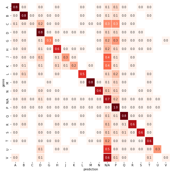
In-sample classification accuracy comes in at ~82%. This means that our model can correctly explain approximately 82% of the generes based soley on word usage. Not bad at all. If we unpack this overall accuracy by genere as shown in the heatmap below, we start to see that not all genre has equal performance. Accuracy ranges from as high as 96% for genre P (Language and Literature) to as low as 2% for genre V (Naval Science).
If we look at accuracy vs. sample count per genre, we can see that genres with lower sample count tend to have lower accuracy. This makes sense as with lower sample count, there is lower variance to learn patterns from compared to other genres. This also tells me that the overall accuracy of 80% is mostly driven by books that are represented more in the sample, which also makes sense.
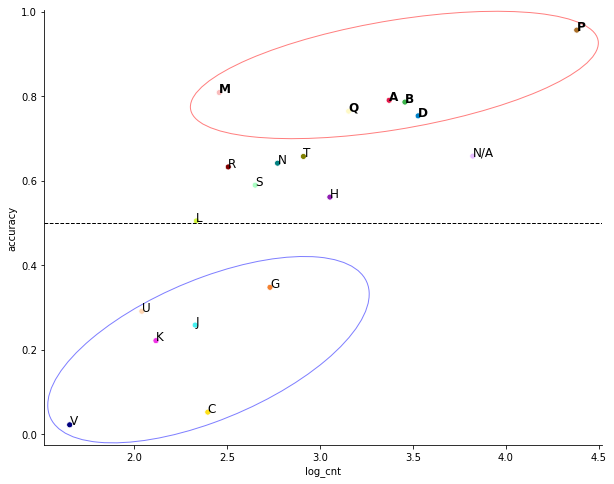
The red circled genres all have higher than 75% accuracy. Genre P (Language and Literature) has the highest accuracy at 96% and genres M(Music) and Q(Science) show great accuracies of 81% and 76% respectively despite their smaller sample size. Music genre is especially impressive and was also highlighted in the t-SNE chart above as seeming to have a strong pattern based on word usage. D is World History; B is Philosophy, Psychology and Religion; A is General Works; and Q is Science.
Genres G (Geography, Anthropology, and Recreation), U(Military Science), J(Political Science), K(Law), C(Auxiliary Sciences of History), and V(Naval Science) in the blue circle all have lower than 50% accuracy. Again, this might be due to lower sample size, or because our Bag-of-Words classification approach is “context-unaware”. Similar set of words are used in these genres as others, but the distinguishing pattern could be in what order or in what combinations different words are used. Our current approach doesn’t pick up patterns like that.
The real classification: 10-fold cross validation (out-of-sample accuracy)
Let’s see how robust our result of ~80% overall acccuracy holds up in out-of-sample classification, that is can we predict the generes of completely new books based on other books? I’ll run this 10 times, each time using a non-overlapping 90% sample of our data to predict the genre of the other 10% as shown below. Each time, approximately 41,000 books are used to predict the genre of 4,600 books.
11:08:48: Testing fold 0 w/ 41204 training set and 4588 test set...
11:09:28: Testing fold 1 w/ 41207 training set and 4585 test set...
11:10:09: Testing fold 2 w/ 41208 training set and 4584 test set...
11:10:54: Testing fold 3 w/ 41210 training set and 4582 test set...
11:11:34: Testing fold 4 w/ 41212 training set and 4580 test set...
11:12:12: Testing fold 5 w/ 41214 training set and 4578 test set...
11:12:52: Testing fold 6 w/ 41216 training set and 4576 test set...
11:13:35: Testing fold 7 w/ 41217 training set and 4575 test set...
11:14:13: Testing fold 8 w/ 41219 training set and 4573 test set...
11:14:57: Testing fold 9 w/ 41221 training set and 4571 test set...
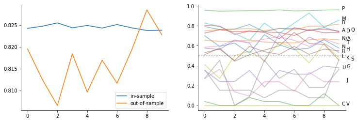
Below are charts summarizing the overall and by genre accuracy for eath of the 10 iterations. First chart shows overall accuracy of the model where 90% of sample is fit (in-sample) and the prediction (out-of-sample classification) accuracy of when this model is applied to new data (the other 10 %) to predict the genre. Second chart breaks down the overall out-of-sample classification accuracy by genre.
- First chart shows that the in-sample and out-of-sample accuracy is pretty close to each other. This is good as it indicates that we are not over-fitting to sample data. Consistent out-of-sample accuracy of around or over 80% seems pretty good as well.
- Second chart tells us that accuracy by genre is also pretty stable over the 10 iterations. This is good as well as it indicates that our model is general enough and our predictions are not sensitive to different sample.
Conclusion
Honestly, I was surprised that the classification accuracy came out pretty well (consistently around ~80%) at first take with basic text cleaning and no hyper-parameter tuning at all. This probably indicates that there is a stronger pattern in text data relative to what I initially expected in terms of which genre it belongs to. Identifying genre of a book might be a trivial task for human beings, as you probably know what type of book it is by reading though a few pages. I do not know of a reasonable human performance benchmark though so we can’t say for sure that this is necessarily the case. One thing for sure is that humans cannot read through ~45,000 books within a matter of seconds and determine the genre of them nor quantify their rationale.
There are more things I can do to improve prediction accuracy.
- I can do some work around hyper-parameter tuning
- Use non-linear models for classification such as Random Forest/XGBoost
- Use a fundamentally different approch to constructing text data through word embeddings compared to the relatively simplistic Bag-of-Words approach. This approach would use more sophisticated models such as word2vec or the state-or-art BERT.
These are quite some work, and I may pursue a few of these when I have time in the future. For now, I’m pretty happy with my 80% overall accuracy :).
Cleaning and preparing text data
Cleaning and preparing text data was very time consuming (~2 weeks) and is a very important process in NLP that can significantly affect prediction performance. I’ve cut some corners here and there, but below is an overview of how I prepared text data from the ~45,000 Project Gutenberg books that logistic regression is fit on. Please read through if you’re interested in the more granular technical details on text data preparation.
- Using
spaCy, tokenize, remove stop words and puncuations, and lemmatize. This results in a corpus of ~9.7 million words. There’s probably a lot of words/phrases that didn’t get parsed/cleaned correctly. Let’s keep going on though. - Trim down corpus by removing words that occur in less than 1% and more than 70% of the books. This results in a significantly reduced corpus of 300k words. This is done to remove “outliers” to the extent they do not inform overall patterns. Cutoffs were determined based on how rapidly the corpus size declined with respect to these lower/higher-end cutoff parameters. I chose 1% and 70% when the rapid decline seemed to taper off.
- Construct document-term matrix using
sklearn.feature_extraction.text.TfidfVectorizer - Reduce dimensionality from 300k to 300 (factor of 1,000 which is randomly selected) using
sklearn.decomposition.TruncatedSVDby taking the left singular matrix from the Singular Vector Decomposition (SVD) factors. This is done to i) smoothen out the sparisity of the document-term-matrix and 2) reduce the dimension for accelerated computation. Right singular matrix of SVD can also be used for latent semantic analysis (LSA).